The program lidar_ozone_actris_v01.py#
Major steps of the LIDAR processing#
Overview#
The program is organized around two major processing phases, each composed of several steps.
LIDAR raw data are photon counts measured by detectors, and are therefore strongly affected by the instrumental chain. The goal of the first phase, called pre-processing, is to remove instrument-related effects: sky/background subtraction, detector desaturation (saturation correction), and geometric factor correction. After this phase, the physical nature of the signal remains the same as at the input, but cleaned from instrumental biases.
The second phase, simply called processing, converts the measured physical quantity into the target geophysical variable. For an ozone DIAL, this means converting received photon counts into ozone number density (or concentration).
The pre-processing is instrument-specific, while the processing should be identical for a given retrieved geophysical quantity (e.g., ozone), regardless of the instrument.
Tip
Keep the distinction clear in your XML: pre-processing parameters depend on the hardware; processing parameters should be driven by the targeted geophysical product.
Background, detector noise, and induced signal#
We group three effects under “background”:
Sky background light: sunlight, moonlight, starlight, artificial light from cities and nearby buildings. This is broadly a (wavelength-dependent) white noise, approximately independent of altitude. Its time variability is generally slow but non-zero.
Detector dark noise / electronic background: even in complete darkness the detector and acquisition electronics produce counts. This is typically white noise, detector-dependent, and altitude-independent. In theory it is stable in time, but aging can change its level; periodic checks are recommended.
Induced signal (afterpulsing / persistence): a light-dependent contribution where photons captured by the detector are released later. This becomes noticeable when the received signal is large. Unlike white noise, this component depends on altitude.
In the “background” step, we aim to remove these three contributions together. In theory, a simple average over a far-range window is enough; however, because of induced signal, a (weighted) linear regression on the far-range background is often preferred to correct the induced component. The fitted slope should be small; a large slope indicates significant induced signal or another issue.
Warning
A steep regression slope in the background fit is a red flag. Check for afterpulsing, bright clouds, or stray light. Consider narrowing the background altitude window or using robust (weighted) regression.
Note
Keep the background window away from cloud layers and from the maximum range where digitizer artifacts may appear.
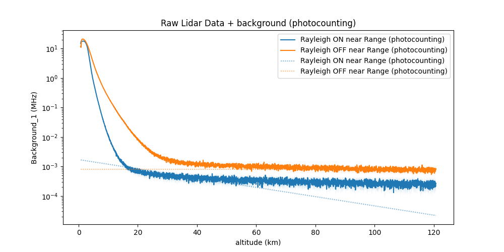
Example of background correction#
Desaturation#
Detectors saturate when they receive too much light: beyond a threshold they no longer count linearly, and even before hard saturation they undercount photons. Several parametric models exist to correct for this behavior (e.g., Pelon model), with parameters that may evolve as the detector ages.
Warning
Saturation parameters are instrument- and channel-dependent and may drift with time. Recalibrate regularly using controlled acquisitions or low-altitude cloud returns.
Tip
After desaturation, compare corrected signals to the simulated/expected dynamic range to ensure consistency.
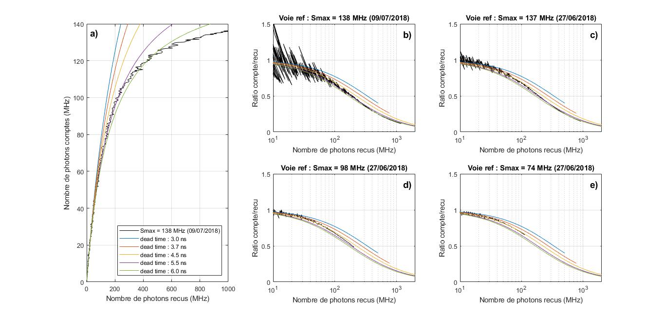
Study of signal desaturation using the Müller method#
Geometrical factor#
The geometrical factor quantifies how well the telescope field of view overlaps the laser beam. It is 0 when there is no overlap (laser out of the FOV), 1 when fully overlapped, and in-between for partial overlap.
Note
Overlap can be provided by measurement, by optical modeling, or estimated during clear, aerosol-free conditions using molecular returns.
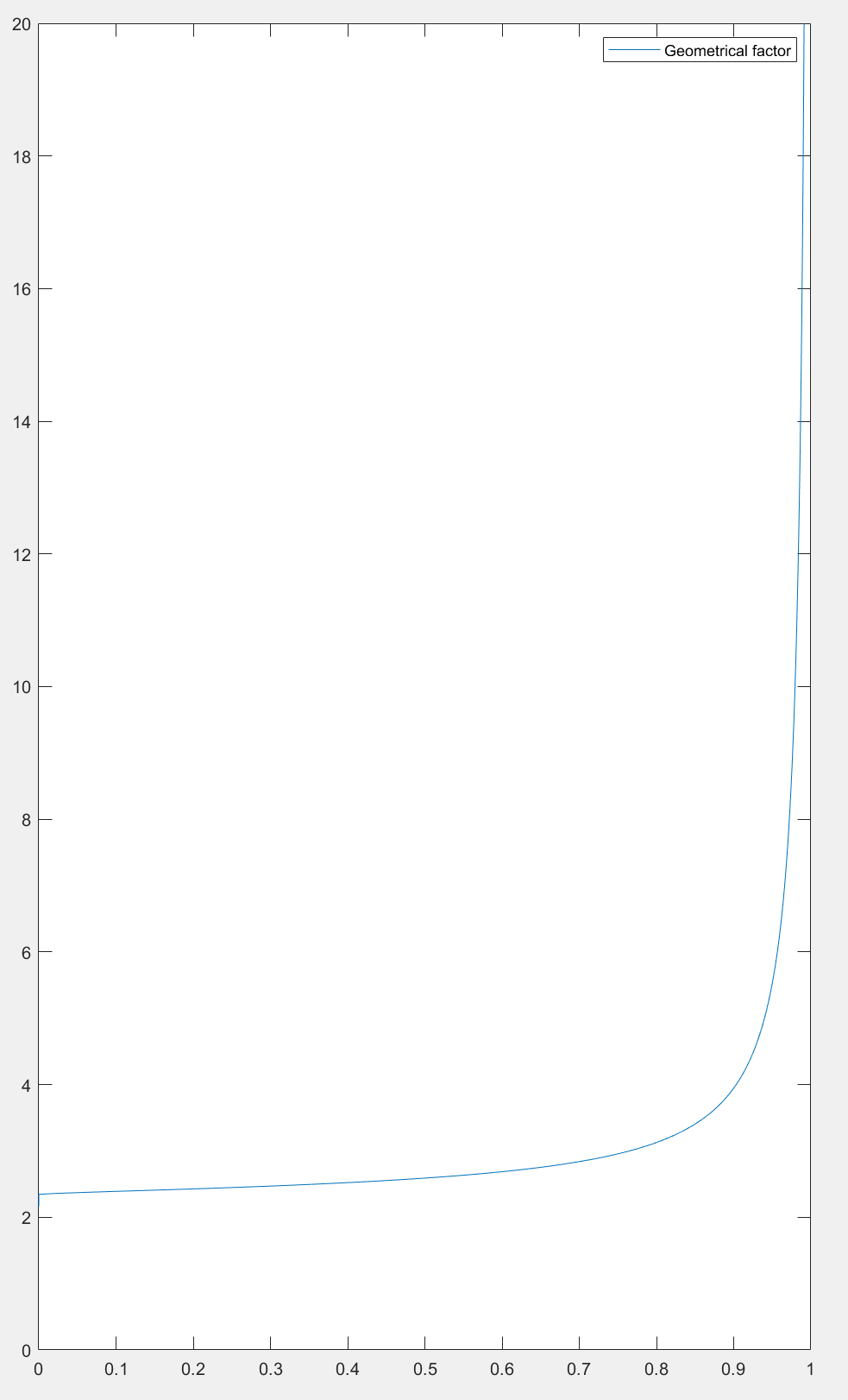
Example of a geometrical factor#
Signal gluing (channel merging)#
Because detectors operate over limited dynamic ranges, multiple channels are often used to cover the full altitude range. Gluing (merging) combines overlapping channels into a single continuous profile.
Tip
Use overlap ranges with stable SNR and no saturation on either channel. Track and apply vertical shifts if timing offsets or bin origins differ.
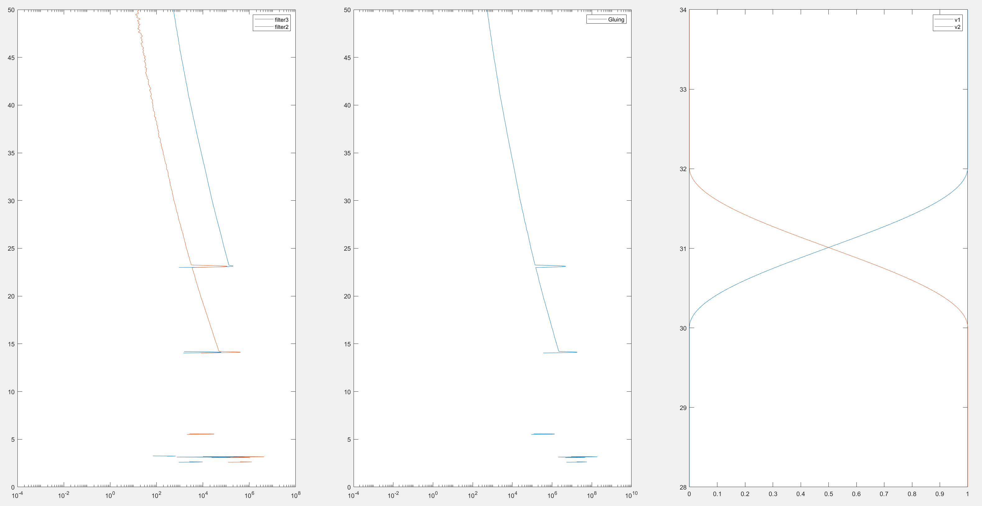
Example of channel gluing between a high-range (orange) and a low-range (blue) channel. Left: raw channels; middle: glued signal; right: applied merging weights (here, cosine/sine-squared). A vertical shift of the high-range channel relative to the low-range one is also applied.#
Signal filtering#
Filtering reduces noise and increases the usable altitude range. Because noise is signal-dependent (and thus altitude-dependent), an altitude-adaptive filter width is often used: at low altitudes (high SNR) we use short windows (high resolution); at high altitudes (low SNR) we use longer windows (lower resolution).
Filtering trades noise for resolution: averaging over more points reduces noise but lowers the number of independent samples.
Warning
Excessive smoothing can bias gradients and degrade the DIAL derivative. Validate window lengths against known structures (e.g., tropopause, aerosol layers).
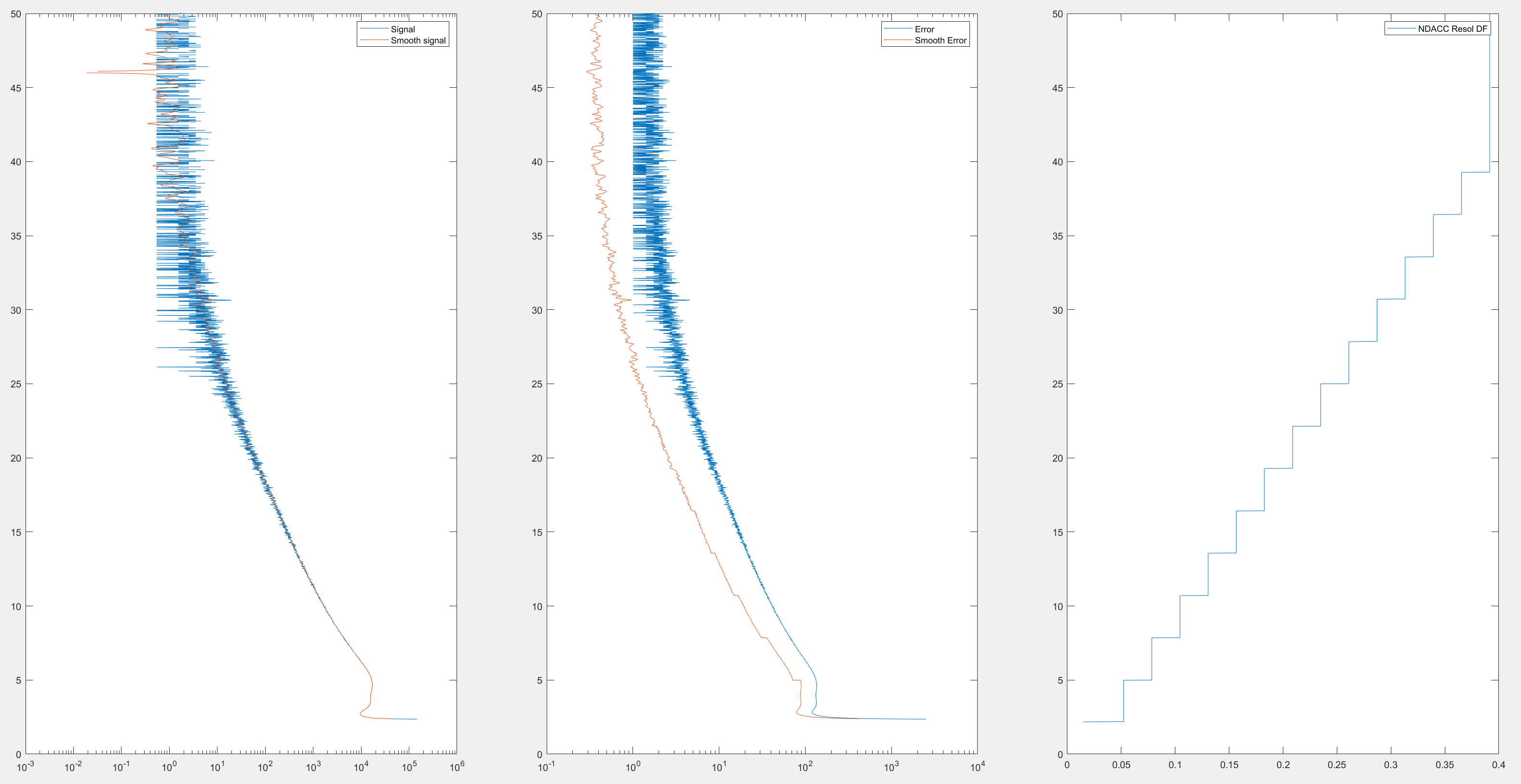
Example of filtering. Left: filtered (orange) vs raw (blue) signal; middle: reduced uncertainty for the filtered signal; right: effective vertical resolution increasing with altitude (e.g., from 50 m at 4 km to ~400 m at 40 km).#
Aerosol retrieval#
We retrieve aerosol backscatter using the Klett method. This applies to Rayleigh-Mie channels at wavelengths not perturbed by absorbing gases (e.g., not the ozone ON channel).
A common diagnostic is the backscatter ratio (BSR): the ratio of total backscattered signal to purely molecular backscatter. A BSR of 1 indicates no aerosols; values > 1 indicate aerosol presence. Values < 1 suggest inconsistencies or errors.
Note
Choose a molecular reference altitude where aerosol load is minimal (e.g., upper stratosphere), or provide an external reference if needed.
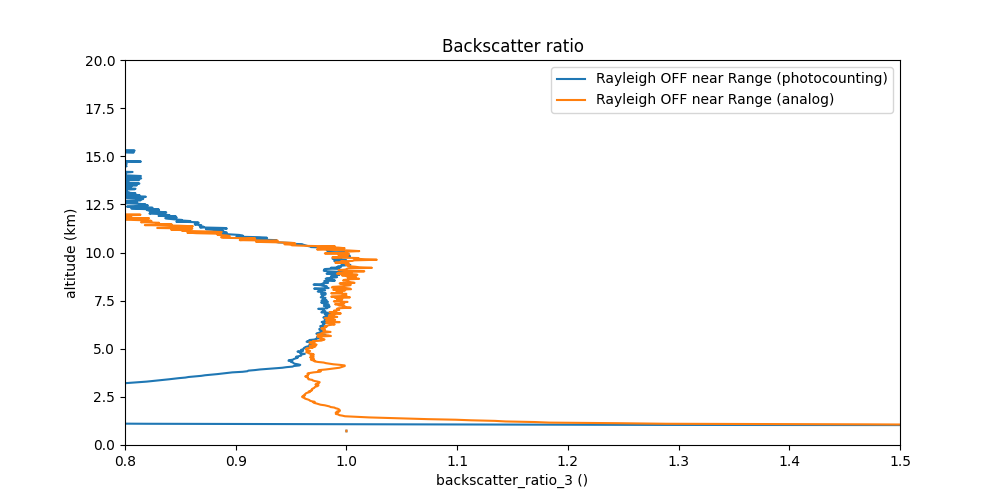
Example of backscatter ratio#
Ozone retrieval#
Starting from the LIDAR equation for a Rayleigh channel:
with:
\(P\): received power (counts)
\(\lambda_e\): emission wavelength
\(\lambda_r\): reception wavelength
\(z\): altitude
\(K\): instrumental constant
\(A\): solid angle (or overlap term)
\(\beta\): volume backscatter coefficient
\(\tau_i\): optical depth of atmospheric constituent \(i\) (major gases N2, O2, aerosols, and minor constituents e.g., O3, SO2, …)
Optical depth is the vertical integral of extinction:
Define the range-corrected signal \(Pz2\):
Taking the derivative of the logarithm:
For the two DIAL wavelengths \(\lambda_\mathrm{on}\) and \(\lambda_\mathrm{off}\), we have:
For compactness, define:
Subtracting the two equations in (1):
Using \(\alpha_i(\lambda, z) = \sigma_i(\lambda, z)\, n_i(z)\):
with
Finally, the main DIAL equation becomes:
Solving for ozone number density:
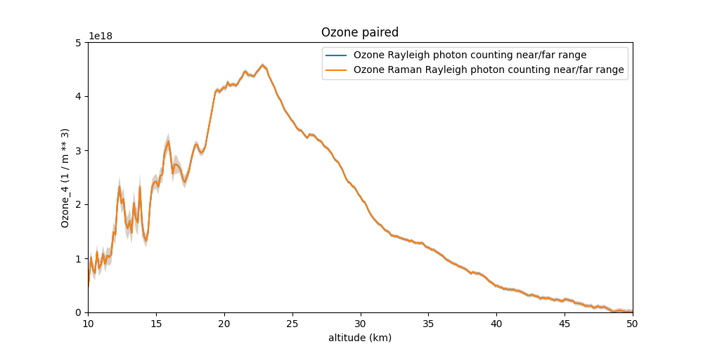
Example of an ozone profile#
Warning
The derivative operators amplify noise. Ensure adequate filtering and report the effective vertical resolution together with ozone profiles.
Temperature retrieval#
Temperature can be derived from the hydrostatic equation combined with the ideal gas law using pressure and density profiles (or via Raman channels when available). In this pipeline:
Pressure is obtained by integrating hydrostatic balance from a reference level using density or temperature climatologies.
Temperature is then computed from the ideal gas law once number density (or ozone-corrected molecular density) is known.
Outputs: - Temperature profile \(T(z)\) in K - Associated uncertainty (propagated from pressure/number-density errors) - Effective vertical resolution
Note
Provide a reference pressure/temperature at a known altitude (e.g., station level or radiosonde). Consistency with auxiliary data (radiosonde, NWP) should be checked.
How lidar_ozone_actris_v01 works#
Calling the function#
The function lidar_ozone_actris_v01 accepts two arguments: the parameter file and an optional date to process. The date can also be provided in the parameter file. This enables running the program with one parameter file per station.
The parameter file can be a string (absolute or relative path) or a ParametersFromXml object (See Parameter file in xml).
def lidar_ozone_actris_v01(
    path_parameters_file: str | ParametersFromXml | None = None,
    dt: str | date | None = None
) -> Lidar | None:
    """
    Data processing for DIAL ozone LIDAR, ACTRIS.

    :param path_parameters_file: path to the parameters file (default: None)
    :type path_parameters_file: str or ParametersFromXml or None
    :param dt: date to process (default: None)
    :type dt: str or datetime.date or None
    :return: the Lidar object
    :rtype: Lidar or None
    """
Initialization#
Return None if path_parameters_file is None. Returning None (instead of raising) allows automated scheduling/retries, as discussed later.
########
# Init #
########
if path_parameters_file is None:
    return None
Creating the Lidar object#
The whole pipeline is driven by the Lidar class. We initialize it with the two inputs of lidar_ozone_actris_v01. The object stores all datasets (LIDAR, auxiliary data, processing results, etc.) and exposes processing methods. Data are stored using NetCDF conventions.
#####################
# 0. Parameter File #
#####################
lidar = Lidar(path_parameters_file, dt)
If the date is provided as a parameter, it is saved to the XML at:
<Dial>
    <Read>
        <date_to_process>
            <date type="date" format_date="iso"></date>
        </date_to_process>
    </Read>
</Dial>
ISO format is YYYY-MM-DD (e.g., 2023-03-28).
Importing LIDAR data#
First, we import the raw LIDAR data into the Lidar object. These data define the core coordinates of the NetCDF file: altitude and time.
#############################
# 1. Reading Raw Lidar Data #
#############################
lidar.import_lidar_data()
Configure this step in XML:
<Dial>
    <Read>
        <Lidar_files>
            <filenames type="relativepath">pathname_lidar</filenames>
            <format>Teslas</format>
            <Signal_type type="int">
                102, 103, 100, 101, 104, 105
            </Signal_type>
        </Lidar_files>
    </Read>
</Dial>
The program will read pathname_lidar, using the specified format (here, Teslas) and the Signal_type values for each channel. The meaning of Signal_type is described in Signal types (Signal_Type).
Multiple files can be provided in filenames, separated by a delimiter (default ,, configurable):
<Dial>
    <Read>
        <Lidar_files>
            <filenames type="relativepath" delimiter=";">
                pathname_lidar_1;pathname_lidar_2
            </filenames>
        </Lidar_files>
    </Read>
</Dial>
For date-dependent directory structures, filenames can be split into sub-fields. In the example below the program looks for files matching: Configuration_files/Main_files/Lidar/sho240328*.s* (i.e., empty directory date, and file date format %y%m%d):
<Dial>
    <Read>
        <date_to_process>
            <date type="date" format_date="iso">2024-03-28</date>
        </date_to_process>
        <Lidar_files>
            <filenames type="relativepath">
                <directory check="directory" type="relativepath">
                    Configuration_files/Main_files/Lidar
                </directory>
                <directory_date_format></directory_date_format>
                <data_name_prefixe>sho</data_name_prefixe>
                <data_name_suffixe>*.s*</data_name_suffixe>
                <data_name_date_format>%y%m%d</data_name_date_format>
            </filenames>
        </Lidar_files>
    </Read>
</Dial>
Input data units can be specified: “photocounting” (default) or “MHz”:
<Dial>
    <Read>
        <unit_photocounting>MHz</unit_photocounting>
    </Read>
</Dial>
To discard some channels from the raw file, use Remove_channel with the corresponding Signal_type values:
<Dial>
    <Read>
        <Remove_channel type="int">101</Remove_channel>
    </Read>
</Dial>
If raw channels have different range resolutions, resampling is needed. Forcing a target resolution to 15 meters:
<Dial>
    <Read>
        <ForceResolution type="float" units="m">15</ForceResolution>
    </Read>
</Dial>
An electronic delay (per-channel if needed) can be added to compute the altitude vector:
<Dial>
    <Read>
        <electronic_delay type="float" units="ns">100, 100, 100, 100, 100, 100</electronic_delay>
    </Read>
</Dial>
Importing auxiliary data#
At minimum, the program requires pressure and temperature profiles versus altitude. For plotting and comparisons, ozone-related auxiliary components are also loaded:
############################
# 2. Import Auxiliary Data #
############################
lidar.import_atmospheric_component()
lidar.import_other_atmospheric_component("ozone")
In the XML, configure the Atmosphere_file section. Several models can be stitched by altitude (e.g., radiosonde up to ~30 km, then climatologies). We define multiple modele_X blocks (X is an arbitrary index; for readability, use ascending order):
one or several filenames (same patterning options as for LIDAR files),
file format (e.g., radiosonde, ncep, arletty, MAP85, …),
concatenation order,
fill value,
model-specific variables (e.g., station name for Arletty).
A useful option is time_shift (hours or days depending on your implementation) to offset the datetime used to find files (e.g., use the previous day’s radiosonde with -1).
Example:
<Dial>
    <Read>
        <Atmosphere_file>
            <modele_0>
                <filenames type="relativepath">
                    <directory check="directory" type="relativepath">
                        Configuration_files/Main_files/Atmosphere
                    </directory>
                    <directory_date_format></directory_date_format>
                    <data_name_prefixe delimiter=",">ht, te</data_name_prefixe>
                    <data_name_suffixe>.nmc</data_name_suffixe>
                    <data_name_date_format>%y%m%d</data_name_date_format>
                    <time_shift type="float">0</time_shift>
                </filenames>
                <format>ncep</format>
                <order type="int">1</order>
                <fill_value>nan</fill_value>
                <station_name>OHP</station_name>
            </modele_0>
            <modele_1>
                <filenames type="relativepath">
                    Configuration_files/Main_files/Atmosphere/MAP85_PRE.DAT,
                    Configuration_files/Main_files/Atmosphere/MAP85_TEMn.DAT
                </filenames>
                <format>MAP85</format>
                <order type="int">1</order>
                <fill_value>nan</fill_value>
            </modele_1>
        </Atmosphere_file>
    </Read>
</Dial>
The program also needs ozone absorption cross-sections:
<Dial>
    <Read>
        <Cross_section_file>
            <filenames type="relativepath">
                Configuration_files/Main_files/Ozone_cross_section/O3_CRS_BDM_218K.dat,
                Configuration_files/Main_files/Ozone_cross_section/O3_CRS_BDM_228K.dat,
                Configuration_files/Main_files/Ozone_cross_section/O3_CRS_BDM_243K.dat,
                Configuration_files/Main_files/Ozone_cross_section/O3_CRS_BDM_273K.dat,
                Configuration_files/Main_files/Ozone_cross_section/O3_CRS_BDM_295K.dat
            </filenames>
            <format>Bass And Paur files</format>
        </Cross_section_file>
    </Read>
</Dial>
For plotting references, provide an ozone climatology:
<Dial>
    <Read>
        <Climatology_ozone_file>
            <filenames type="relativepath">
                Configuration_files/Climatology_files/climatology_ozone_ohp.nc
            </filenames>
            <format>netcdf</format>
        </Climatology_ozone_file>
    </Read>
</Dial>
Tip
Ensure consistent units (number density vs. mixing ratio) and wavelength definitions (emission vs. reception) across auxiliary files.
Simulated LIDAR signal#
To validate results and produce figures, a theoretical/simulated LIDAR signal can be generated at each stage:
###########################
# Lidar Signal Simulation #
###########################
lidar.create_simulated_lidar()
Pre-processing#
The pipeline implements three pre-processing steps: background, desaturation, and geometrical factor. They are configured in XML and applied via the Lidar methods:
###############
# Pre-Process #
###############
lidar.background()
lidar.saturation()
lidar.geometrical_factor()
lidar.apply_preprocess()
Example XML:
<Dial>
    <!-- DESATURATION -->
    <Desaturation>
        <Method>pelon, pelon, pelon, pelon, pelon, pelon</Method>
        <Parameters>
            <tau type="float" units="ns">3.7e-9,3.7e-9,3.7e-9,3.7e-9,3.7e-9,3.7e-9</tau>
            <N_cm type="float">77.895,79.84,80.7487,70.1884,60,60</N_cm>
        </Parameters>
    </Desaturation>

    <!-- SKY BACKGROUND -->
    <SkyBackground>
        <Method>Weighted linear regression, Weighted linear regression, Average, Average, Average, Average</Method>
        <Parameters>
            <alt_min units="m" separator=",">100220,92270,87620,92270,65870,60020</alt_min>
            <alt_max units="m" separator=",">149870,138000,149870,149870,149870,149870</alt_max>
            <order type="int">1,1,0,0,0,0</order>
            <log_regression type="bool">False,False,False,False,False,False</log_regression>
        </Parameters>
    </SkyBackground>

    <!-- GEOMETRIC FACTOR -->
    <GeometricFactor>
        <filenmes relativepath="True"></filenmes>
        <format>mrd</format>
    </GeometricFactor>
</Dial>
Aerosol processing#
To diagnose aerosol presence and correct ozone retrievals when needed, the aerosol backscatter profile is computed:
####################
# Aerosols Process #
####################
lidar.aerosols_process()
Example XML:
<Dial>
    <Aerosols>
        <altitude_max type="float" units="km">40</altitude_max>
        <altitude_ref type="float" units="km">25</altitude_ref>
        <beta_aero_ref type="float" units="m**-1">0</beta_aero_ref>
        <method>Klett</method>
    </Aerosols>
</Dial>
Ozone profile by the DIAL method#
For ozone, we filter (and differentiate) the signals, glue high/low range measurements, perform the DIAL retrieval, and finally glue Rayleigh and Raman channels where applicable:
#################
# Ozone Process #
#################
lidar.filtering()
lidar.glue(name_param_tag="MergingSlope")
lidar.ozone_process()
lidar.glue()
Example XML:
<Dial>
    <Filtering>
        <parameters>
            <filter_name>Savitzky-Golay</filter_name>
            <mode>dial poly</mode>
            <ncan1>3,3,4,4,5,5</ncan1>
            <ican1>120,120,120,120,60,60</ican1>
            <ncan2>35,35,30,30,40,40</ncan2>
            <ican2>300,300,300,300,200,200</ican2>
            <alt_unit>km</alt_unit>
        </parameters>
        <resolution_methodology options="df,ir,origin" multiple_option="True">df, ir, origin</resolution_methodology>
    </Filtering>

    <MergingSlope>
        <channel_1 type="int" separator=",">100, 101</channel_1>
        <channel_2 type="int" separator=",">102, 103</channel_2>
        <method separator=",">linear, linear</method>
        <shift type="int" separator=",">0, 0</shift>
        <alt_min type="float" units="km" separator=",">17.12,17.12</alt_min>
        <alt_max type="float" units="km" separator=",">18.02,18.02</alt_max>
    </MergingSlope>

    <MergingOzone>
        <channel_1>132</channel_1>
        <channel_2>136</channel_2>
        <method>linear</method>
        <shift>0</shift>
        <alt_min units="km">9.02</alt_min>
        <alt_max units="km">10.07</alt_max>
    </MergingOzone>

    <Ozone>
        <binomial_filter type="int">2</binomial_filter>
    </Ozone>
</Dial>
Validity domain#
Define and enforce a validity mask based on:
Altitude range: where SNR and overlap are acceptable (e.g., above near-field overlap and below max range).
SNR thresholds: per-channel minimum SNR for derivative operations (DIAL).
Filtering bounds: maximum window length to avoid over-smoothing of sharp gradients.
Cloud screening: remove saturated cloud returns and strong multiple scattering layers.
Consistency checks: ON/OFF consistency; Rayleigh vs Raman ozone where available.
Warning
Report the effective vertical resolution and data flags with each product. Users must not interpret profiles beyond the stated validity domain.
Partial ozone columns#
Compute partial columns by vertically integrating number density over a layer \([z_1,z_2]\):
Outputs: - Partial column in DU (Dobson Units) or molecules·cm⁻², - Random uncertainty (propagated from profile errors), - Systematic terms (e.g., cross-section, calibration).
Tip
Provide a standard set of layers (e.g., 0–6 km, 6–12 km, 12–20 km, …) for comparison with other datasets.
Adding a geometric factor#
If an external overlap (geometrical factor) file is available:
Specify file path and format in the GeometricFactor XML section.
Ensure the overlap altitude grid matches (or is interpolated to) the LIDAR grid.
Validate using clear-air nights and compare with molecular simulations.
Warning
Mismatched overlap functions can introduce large low-altitude biases. Always verify before publishing results.
Data export#
Generated files typically include:
NetCDF profiles: altitude, time, ozone number density, uncertainties, effective resolution, flags, auxiliary (T, P), metadata (instrument, wavelengths, processing version).
CSV summaries: quick-look metrics (layer columns, tropopause ozone, QC flags).
Logs: processing steps, warnings, parameter hashes for reproducibility.
Note
Conform to CF/ACDD-style metadata where possible (units, standard_name, long_name). Include software version and git commit to ensure traceability.
Running from bash#
To do